What you'll learn in this lesson
- ✓ What cells, rows, and columns are — and why they matter
- ✓ How to read and use Excel cell addresses (like A1, B3, C10)
- ✓ How to select single cells, entire rows, entire columns, and ranges
- ✓ How to resize column width and row height to fit your data
- ✓ How to insert, delete, hide, and navigate the Excel grid efficiently
Understanding cells, rows and columns in Excel is the single most important thing you'll do as a beginner — because every single action you take in Excel happens inside this grid. Whether you're building a monthly budget, tracking sales figures, or creating a class schedule, you're always working with cells, rows, and columns. Everything else you learn — formulas, charts, formatting — sits on top of this foundation.
Imagine you've just opened Excel for the first time. You see a giant grid of boxes staring back at you, and you think: "What do I even click first?" That feeling is completely normal. Thousands of people start exactly where you are right now.
By the end of this lesson, that grid won't feel intimidating at all. You'll know exactly what every row, column, and cell does — and you'll be able to navigate and control them like a pro. Let's get into it.
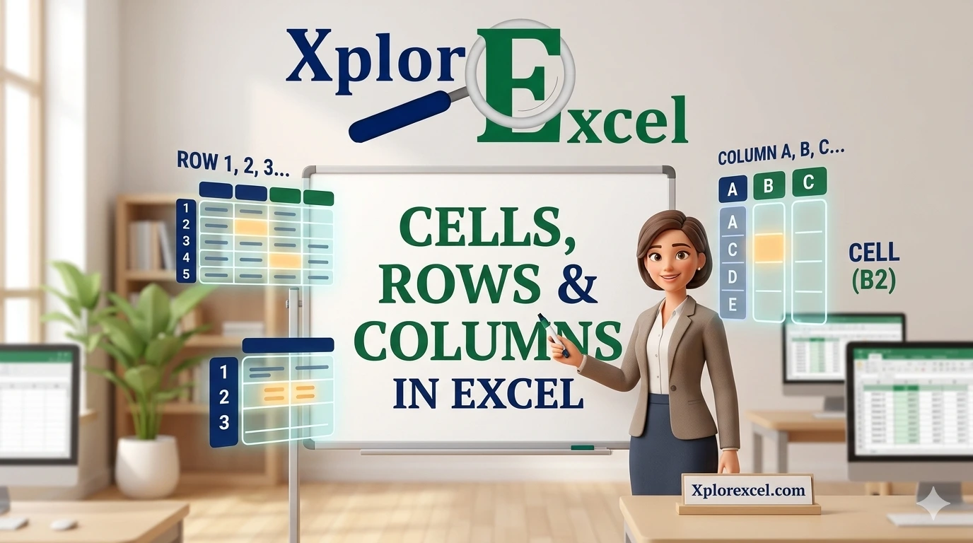
What Are Cells, Rows and Columns in Excel?
When you open an Excel workbook, the first thing you see is a massive grid. That grid is made up of three core building blocks: columns, rows, and cells. Here's the thing — once you understand these three things, the entire Excel interface starts to make sense.
Columns — The Vertical Strips
Columns run vertically — top to bottom — across your spreadsheet. They are labeled with letters: A, B, C, D… all the way to Z, then AA, AB, AC… and so on up to XFD. That's a total of 16,384 columns in a single Excel worksheet. You'll probably never use all of them, but it's good to know the scale you're working with.
You've probably seen the column letters at the very top of the Excel window — that grey bar just above your data. Each letter corresponds to one vertical strip of cells.
Rows — The Horizontal Strips
Rows run horizontally — left to right — across your spreadsheet. They're labeled with numbers: 1, 2, 3… all the way up to 1,048,576. Yes, over one million rows. Excel is built for serious data work, even though most everyday tasks only use a fraction of that capacity.
Row numbers appear along the left edge of the spreadsheet — the grey strip on the far left. Row 1 is always at the top. Many people use row 1 as a header row (for labels like "Name", "Date", "Amount"), then start their actual data in row 2.
Cells — Where the Magic Happens
A cell is the individual rectangular box formed where a column and a row intersect. It's where you actually type your data — a number, a word, a date, a formula, or even nothing at all. Every cell has a unique address, which tells Excel (and you) exactly where that cell lives in the grid.
Trust me on this: once you understand cell addresses, everything about Excel — formulas especially — clicks into place in a way it hasn't before.
Understanding Excel Cell Addresses
Every cell in Excel has a unique cell address (also called a cell reference). The address is always written as the column letter first, then the row number. No spaces, no punctuation — just the column letter followed immediately by the row number.
Cell Address Syntax
[Column Letter] + [Row Number]
A1 → Column A, Row 1
C5 → Column C, Row 5
B12 → Column B, Row 12
AA3 → Column AA (27th column), Row 3
You can always see the address of the cell you're currently clicked on in the Name Box — the small white box on the far left of the Formula Bar (just above your spreadsheet). Click any cell and watch it update instantly.
Cell addresses are the backbone of every Excel formula. When you type =A1+B1, you're telling Excel: "Add whatever is in cell A1 to whatever is in cell B1." That's the power of knowing your cell addresses.
How to Select Cells, Rows and Columns in Excel
Selecting things in Excel is something you'll do hundreds of times every session. The good news: Excel gives you multiple ways to select cells, rows, and columns — from simple single-click selection to powerful keyboard shortcuts that will save you enormous amounts of time.
Selecting a Single Cell
Simply click on any cell to select it. The cell gets a green border (the active cell indicator), and its address appears in the Name Box. You can also jump to any cell instantly by clicking the Name Box, typing the address (like D15), and pressing Enter.
Selecting a Range of Cells
A range is a group of cells. You can select a range by clicking the first cell and dragging your mouse to the last cell. The range address is written as A1:C5 — which means "all cells from A1 to C5." The colon (:) is Excel's way of saying "through."
You can also hold Shift and click the last cell in your range instead of dragging — many people find this more precise.
Selecting an Entire Row or Column
To select an entire row, click the row number on the left. The whole row highlights in blue. To select an entire column, click the column letter at the top. That's it — one click, done.
To select multiple rows or columns at once, click the first row number (or column letter), then hold Shift and click the last one. For non-adjacent selections (rows or columns that aren't next to each other), hold Ctrl instead.
| Selection | Mouse Method | Keyboard Shortcut |
|---|---|---|
| Single cell | Click the cell | Arrow keys to navigate |
| Cell range (A1:C5) | Click + drag | Shift + Arrow keys |
| Entire row | Click row number | Shift + Space |
| Entire column | Click column letter | Ctrl + Space |
| Multiple rows/columns | Click + Shift + click | Shift + click row/col label |
| Entire worksheet | Click top-left corner box | Ctrl + A |
Resizing Column Width and Row Height in Excel
Here's something that trips up almost every new Excel user: you type something into a cell and it looks like it's been cut off or it shows a string of ###### symbols. That's not an error — it just means the column isn't wide enough to display your content. The fix takes two seconds.
Changing Column Width
Hover your mouse over the border between two column letters (for example, between A and B) until the cursor changes to a double-headed arrow. Then click and drag left or right to resize. For a perfect fit, double-click that border and Excel auto-fits the column to its widest content automatically.
Changing Row Height
The same logic applies to rows. Hover over the border between two row numbers on the left side, then click and drag up or down. Double-click to auto-fit.
To resize multiple columns or rows at once, select them all first (click and drag across the column letters or row numbers), then resize any one of them — and all selected ones will resize together.
Step-by-Step: Insert and Delete Rows and Columns in Excel
One of the most common tasks you'll do when working with spreadsheet data is adding or removing rows and columns. Here's exactly how to do it.
How to Insert a Row
- Click the row number where you want the new row to appear. The entire row will highlight in blue. (The new row will be inserted above this selection.)
- Right-click on the highlighted row number to open the context menu.
- Click "Insert" from the menu. A blank row appears above your selected row, and all rows below shift down automatically.
- To insert multiple rows at once, select that many row numbers first (e.g., select 3 row numbers → right-click → Insert → 3 blank rows appear).
- To delete a row, right-click its row number and choose "Delete". The row disappears and everything below moves up.
How to Insert a Column
- Click the column letter where you want the new column. (The new column will be inserted to the left of your selection.)
- Right-click the column letter and choose "Insert".
- A new blank column appears and all columns to the right shift across. Your existing data is safe.
Hiding and Unhiding Rows and Columns
Sometimes you have data you need to keep in the spreadsheet but don't want to display — maybe it's supporting calculations, or a column that's only relevant internally. Excel lets you hide rows and columns without deleting them. The data stays intact; it just becomes invisible.
To hide a row or column: select it, right-click, and choose "Hide". You'll notice the row numbers or column letters skip — for example, if you hide column C, you'll see columns B and D sitting side by side. That's your clue something is hidden.
To unhide: select the rows or columns on either side of the hidden one, right-click, and choose "Unhide". Alternatively, you can hover over the gap between the numbers/letters until you see the resize cursor, then double-click to reveal the hidden content.
Navigating Cells, Rows and Columns in Excel Like a Pro
If you rely on mouse-clicking to move around your spreadsheet, you'll burn a lot of time — especially when working with larger datasets. Learning just a handful of keyboard shortcuts will make navigating the Excel grid dramatically faster. These are genuinely worth memorising.
| Shortcut | What It Does |
|---|---|
Ctrl + Home | Jump to cell A1 (top of spreadsheet) |
Ctrl + End | Jump to the last used cell in your data |
Ctrl + Arrow | Jump to the last filled cell in that direction |
Ctrl + G | Open Go To dialog — type any cell address to jump there |
Tab | Move one cell to the right |
Enter | Move one cell down (confirm entry and advance) |
The Ctrl + Arrow shortcut is especially powerful when you're working with large datasets. Press Ctrl + Down to instantly jump from the top of a column all the way to the last filled cell — no scrolling required.
Real-World Uses: Why Cells, Rows and Columns in Excel Actually Matter
You might be wondering: "OK, this is all useful, but when will I actually need this?" Here are three real-world situations where your understanding of cells, rows, and columns will make a real difference.
1. Building a Monthly Budget
A budget spreadsheet typically puts expense categories in column A (Rent, Food, Transport…), months across row 1 (Jan, Feb, Mar…), and the actual amounts in the intersecting cells. Each cell holds one number. When you need to add a new category, you insert a row. When a new month starts, you insert a column. This is the grid structure doing exactly what it was designed to do.
2. Managing a Contact List or Database
In a contact database, each row is one person. Each column is a type of information: name, email, phone, city, date added. Row 1 is your header row with column labels. Every new contact gets its own row. If you need to add a "Company" column later, you insert a column between existing ones. Understanding the row-per-record, column-per-field structure is fundamental to managing any kind of list in Excel.
3. Calculating Sales Totals with SUM
Say you have sales figures in cells B2 through B13 (one per month). To get the annual total, you'd put your cursor in cell B14 and type: =SUM(B2:B13). Excel adds up everything in that range. Without knowing what B2:B13 means — a range in column B, rows 2 through 13 — that formula is just magic. With this lesson under your belt, it makes perfect sense.
Once you're comfortable with the grid, you'll be entering and editing data directly into these cells. That's exactly what we cover in the next lesson — check out Entering & Editing Data in Excel when you're ready.
💡 Pro Tip: AutoFit All Columns in One Move
Press Ctrl + A to select the entire worksheet, then double-click any column border in the header row. Excel instantly auto-fits every single column to its content width. This is one of the fastest formatting tricks in Excel and saves a lot of time when you're tidying up a messy spreadsheet.
⚠️ Common Mistake: Confusing Columns and Rows
Almost every beginner mixes these up at least once. Remember: columns go up and down (like the columns on a building), and rows go left to right (like rows of seats in a cinema). Columns = letters. Rows = numbers. When you read a cell address like C7 — C is the column (vertical strip), 7 is the row (horizontal strip). Column first, row second. Always.
🎯 Try It Yourself
Open a blank Excel workbook and try these exercises right now — they take less than 5 minutes and will lock in everything from this lesson:
- Click on cell D5. Confirm its address appears in the Name Box top-left.
- Click the Name Box, type G12, press Enter. Watch Excel jump straight there.
- Type your name in cell A1, then type numbers 1–5 down the column in cells A2 through A6.
- Click the column A header letter to select the whole column, then double-click the right border of that column header to auto-fit the width.
- Right-click on row number 3 and insert a new blank row. Then delete it again.
- Press Ctrl + Home to return to cell A1. Notice how instantly it responds.
📚 Go Deeper — Recommended External Resources
These authoritative Excel resources expand on what you've learned in this lesson:
Official Microsoft documentation on working with the Excel grid, rows, and columns.
A comprehensive, well-organised reference for every Excel shortcut — bookmark this one.
Practical, friendly Excel guidance from one of the most trusted Excel educators online.
New to Excel entirely? Before you go further, make sure you've read our Introduction to Excel for Beginners — it covers the workbook interface and will make everything in this lesson click even faster.
← Previous Lesson
Introduction to Excel for BeginnersNext Lesson →
Entering & Editing Data in Excel →