“SUMIF” function is used to know the total of the particular item from the given data.
What is the “SUMIF” Function?
The Excel “SUMIF” Function is used where we need to sum up the value on single criteria i.e. total of the sale of pen, pencil, or notebooks. It can be sum up the value of the cells based on a condition of any Text, number, and logical text. It is also working on matching concepts like VLOOKUP and HLOOKUP but with a condition.
The feature of the “SUMIF” function: –
- With the help of the “SUMIF” function, we can retrieve the total of a particular item from the given data if the condition is matched with the data of the selected cell.
- It helps in applying a particular condition on the given data to get the total value of them.
The logical operator: –
For the “SUMIF” function we can also use follow logical test on the selected data other than the Text and Number.
| Logical Test | Meaning |
| = | Equal to |
| <> | Not Equal to |
| > | Greater than |
| >= | Greater than and Equal to |
| < | Less than |
| <= | Less than and equal to |
Explanation of Function:-
Now, We will explain the Arguments of the Function.
=SUMIF(range, criteria, [sum_range])
range: – Range is that column or row of selected cells on which we want to apply the condition or criteria.
criteria: – This is a condition that we have to apply to the selected cells to get the desired values.
[sum_range]: – Sum range is that range of selected cells, consisting of the values we want to total or sum up. This is optional because in the case where the range and sum_ range are the same. It means we want to make a total of the value when a condition is cleared or matched from the other range of cells, not from the same column or row of the selected range.
Example of Function: –
I will show you, how to apply the whole function. (using optional also).
From the following table get the item-wise value of the total sale amount.
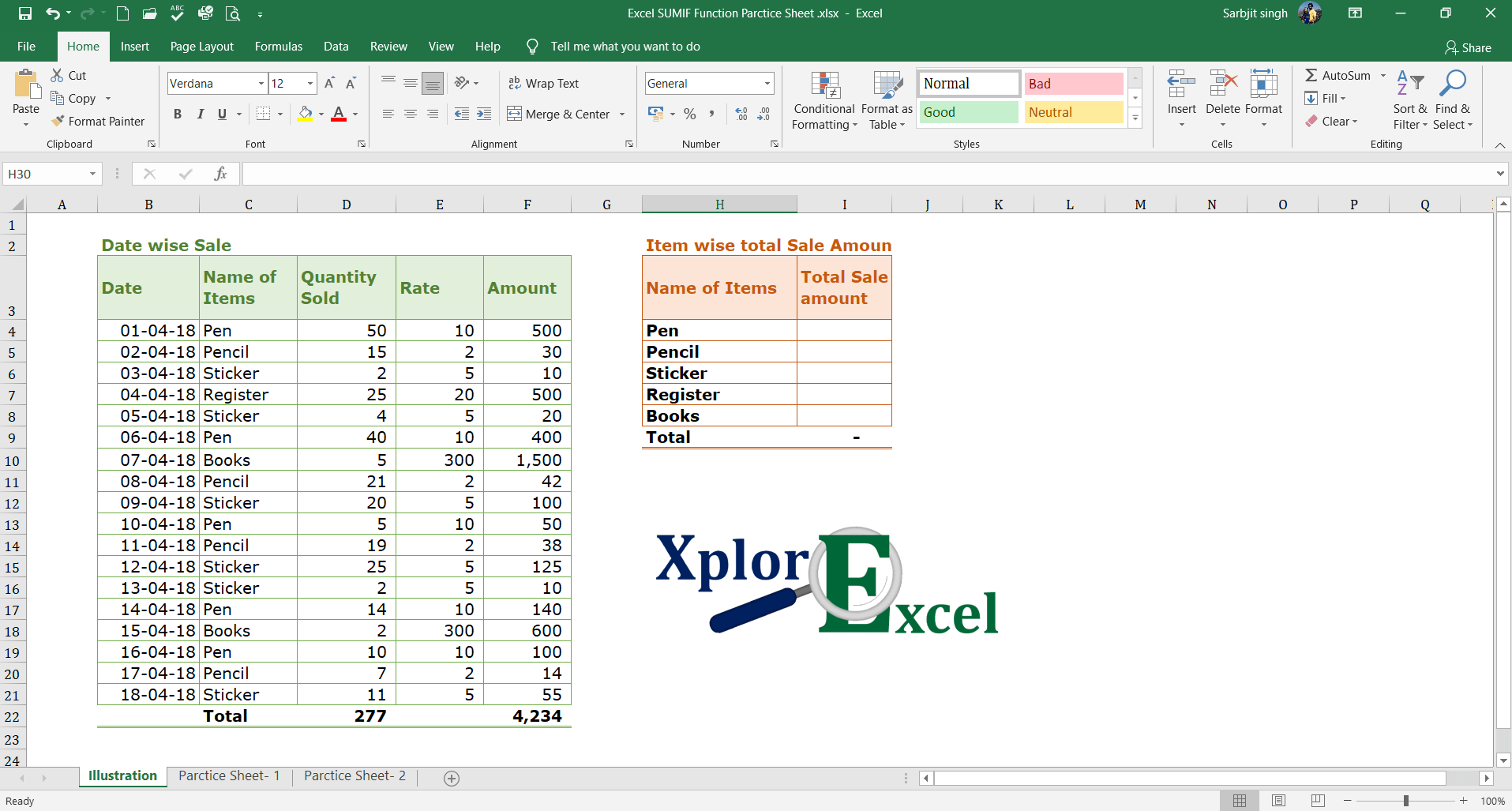
Solution:-
We will Apply the ‘SUMIF’ function and get the result. This is shown in the following steps: –
Step No. 1:-
We will write the “=SUMIF( ” in the column of the result.
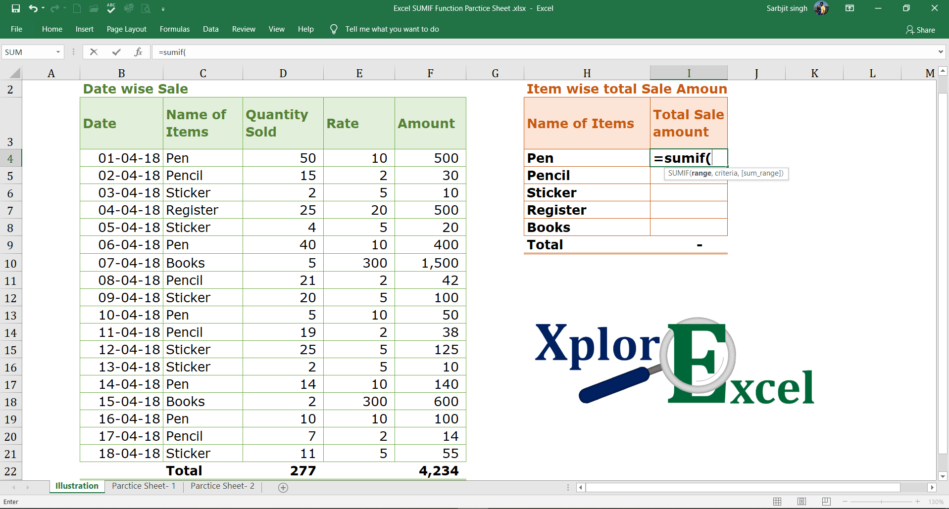
Step No. 2
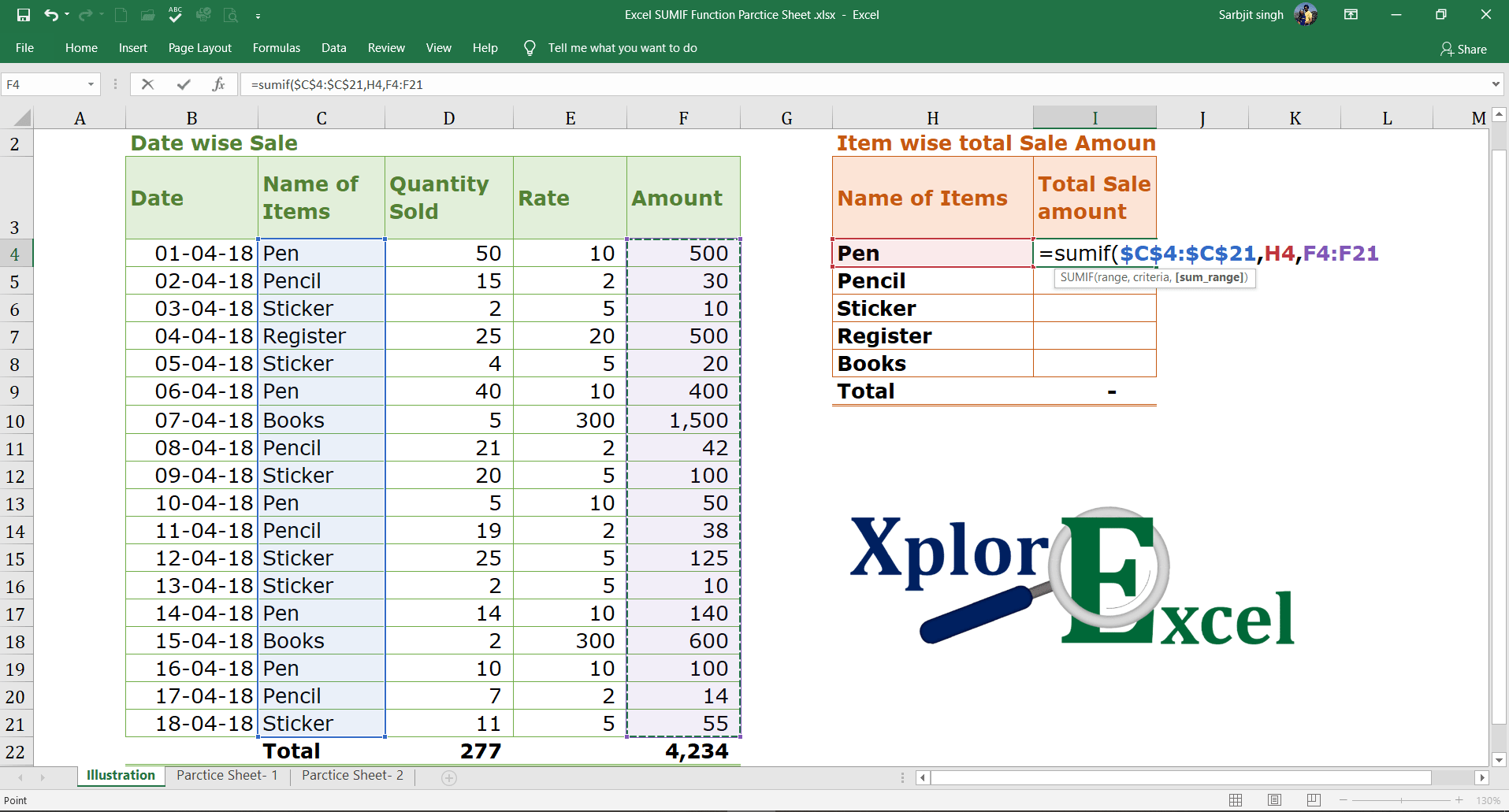
Now select the range on which you want to apply the Condition or criteria.
In an example, we have to sum up the sale amount as per the name of the item. So, we have to apply a condition to the name of the items.
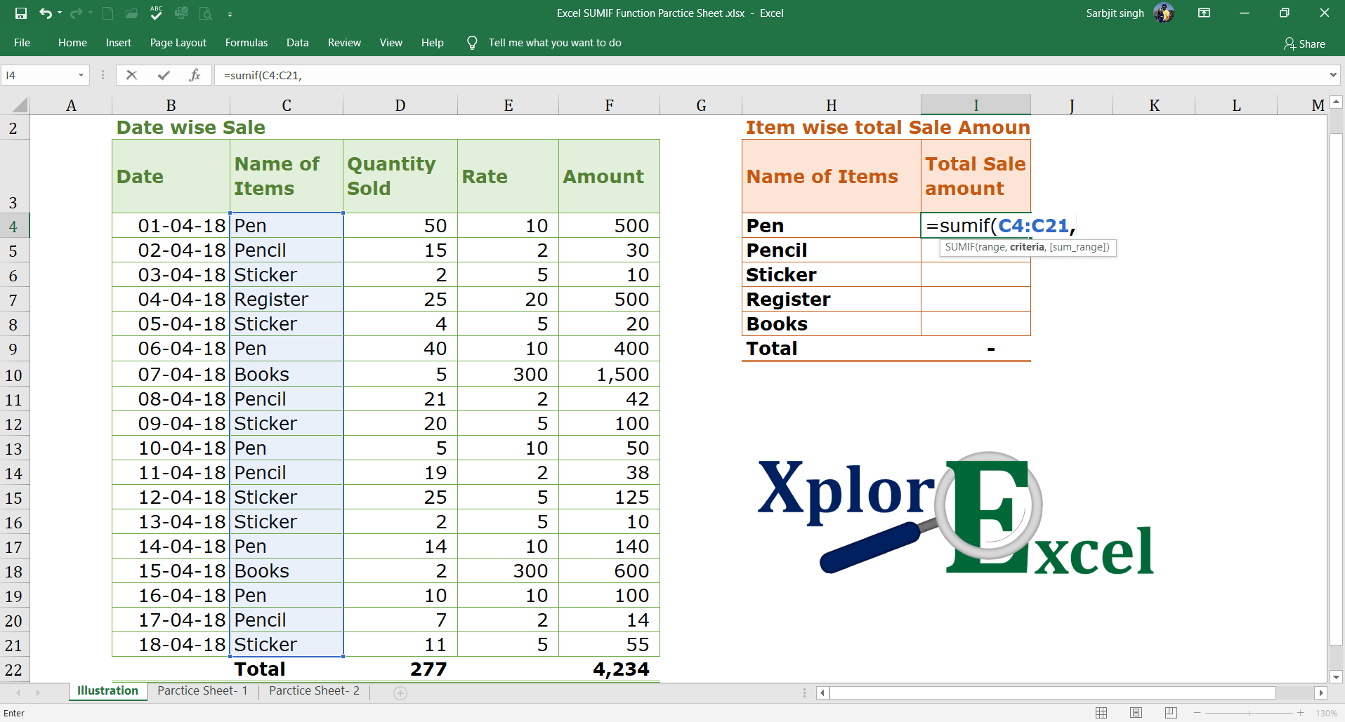
Step No. 3
Now press “F4” to fix the range. it will convert from the C4:C21 to $C$4:$C$21. Because when you copy and paste this formula into another cell the range will remain the same. The excel will find out the condition or criteria from the same cells.

Step No. 4
Now select the Condition or criteria that we want to apply.
In the above example, The names of items are given, and we have to write the total amount in front of them, so we can select the criteria by selecting the cell of the given name.
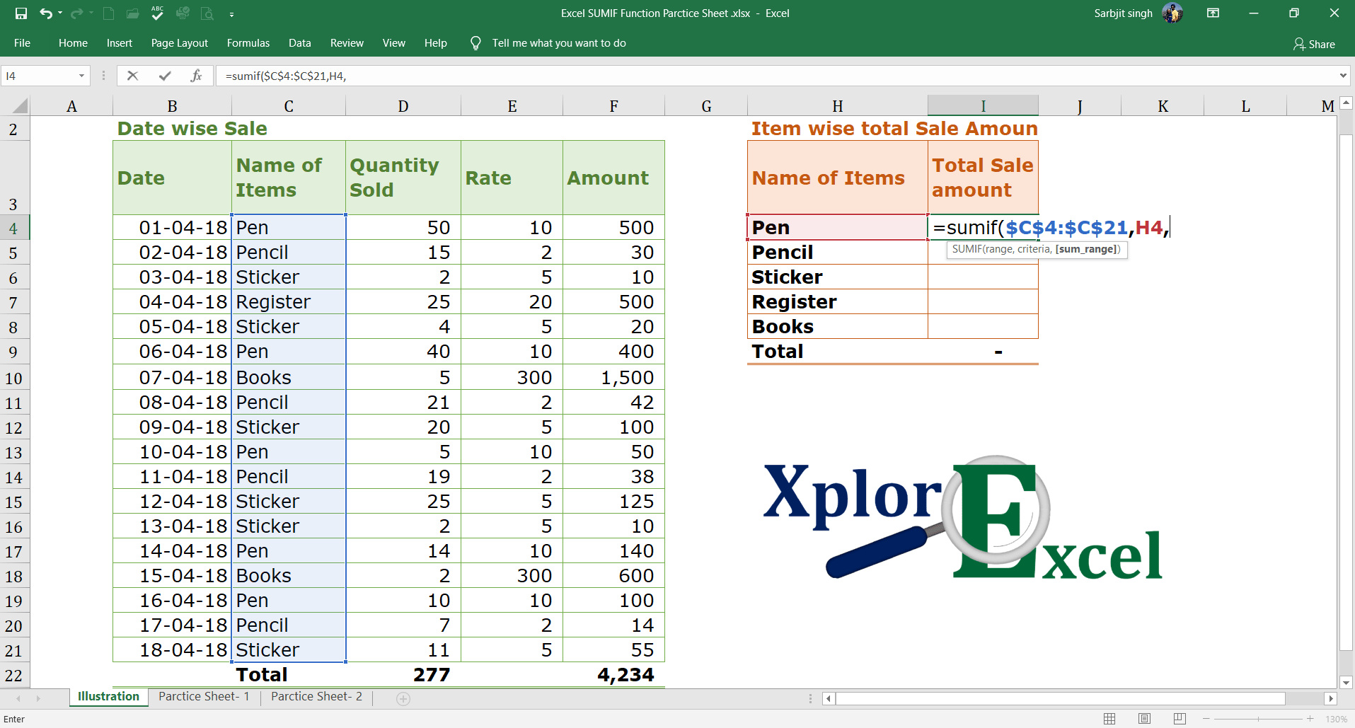
Step No. 5
Now select the range of the cells of which the value we have to sum up.
For example, The total amount of sales dates is given in the “F” column, so we select the cells of the “F” column with the total amount of sales.
Step No. 6
Now press “F4” to fix the range. it will convert from the F4:F21 to $F$4:$F$21. Now when you will copy this formula in another cell then the range remains the same from the excel will find out the condition or criteria.

Step No. 7: –
Now close the brackets:

Step No. 8: –
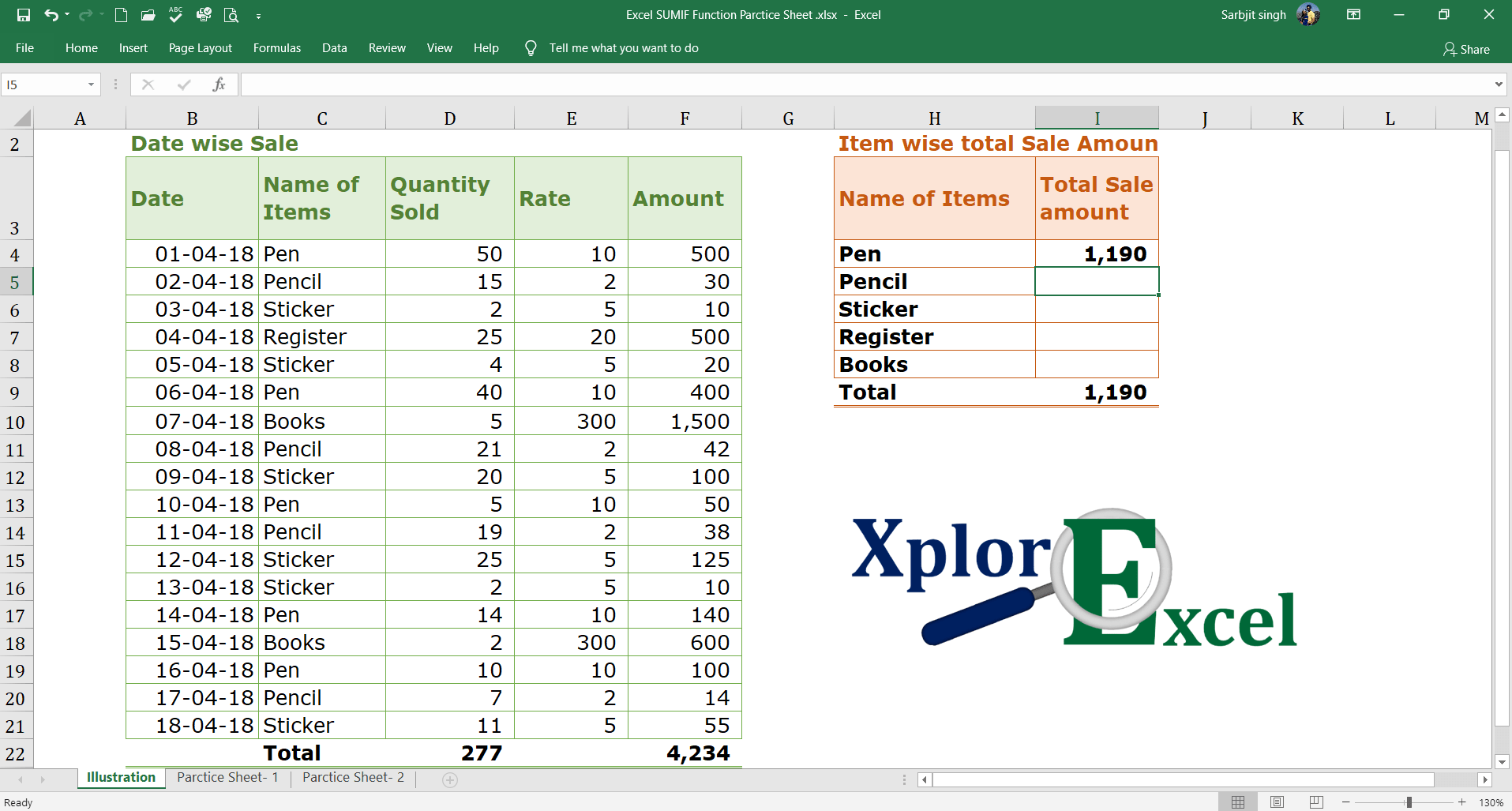
Now, you will get the SUM total of the item named “Pen”:
Step No. 9: –
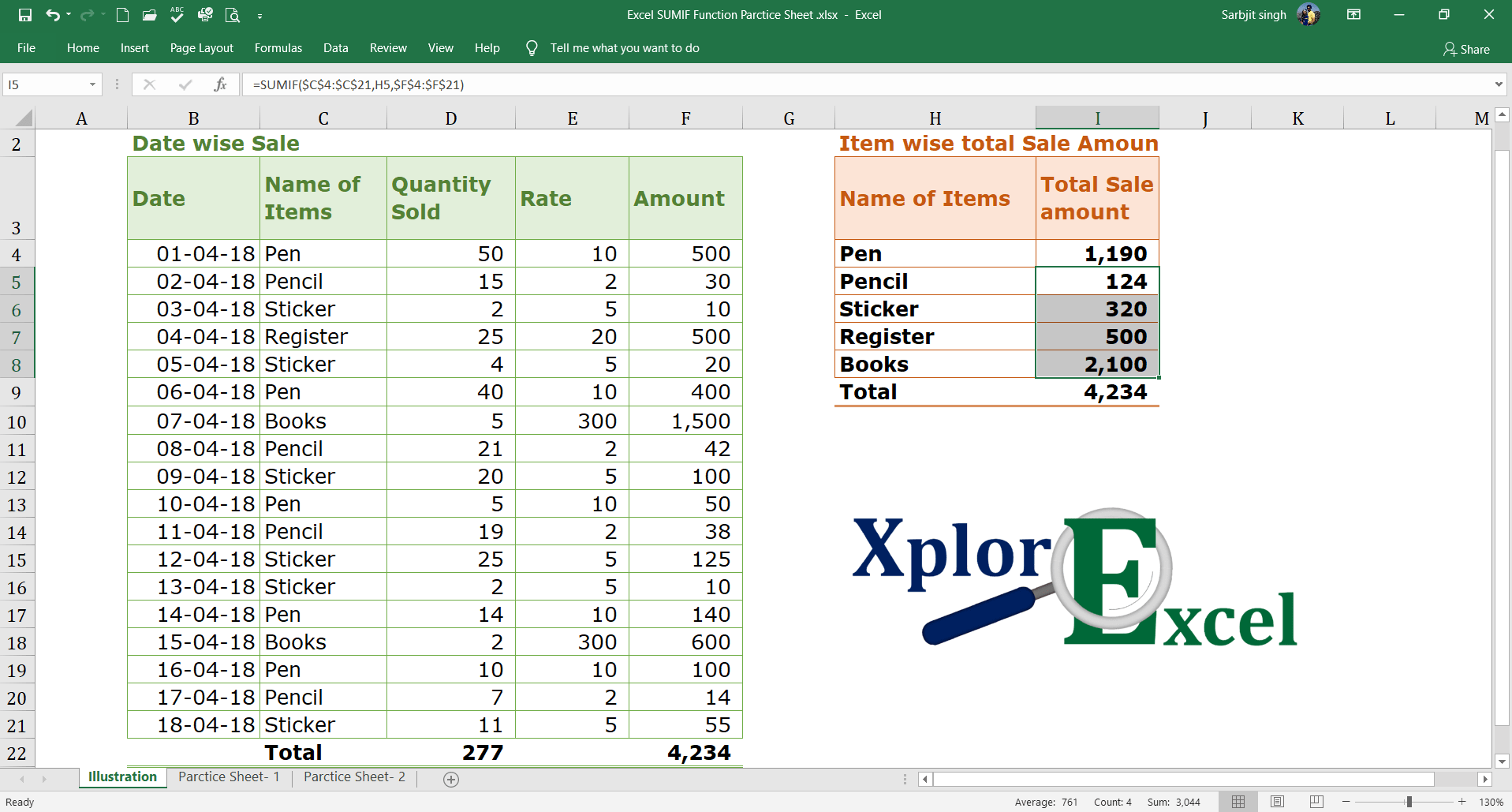
Now, Copy and paste the function in all remaining cells to get the result for all items.
Download the Practice workbook of SUMIF Function
Please Download Practice workbooks from the below links to know how much you have understood the SUMIF Function in Excel:
Check out Other Paid Practice Sheets for Free.
This is all about the SUMIF Function in excel.
Thanks, If you have any confusion about this formula please write a comment in the comment box we reply to you as soon as possible.
Please Share it with your friends and family.
also, write your feedback in the comment box.
to buy Microsoft Excel Click Here.
Also, Check out the following function of excel: –
- How to use VLOOKUP in Excel – free explanation
- How to use HLOOKUP in Excel – free explanation
- IF Function in Excel – Free Explanation with example
- Excel SUMIF Function – Download practice Sheet
- Excel Match Function- Download practice Sheet
- Excel Index Function – Download Practice Sheet
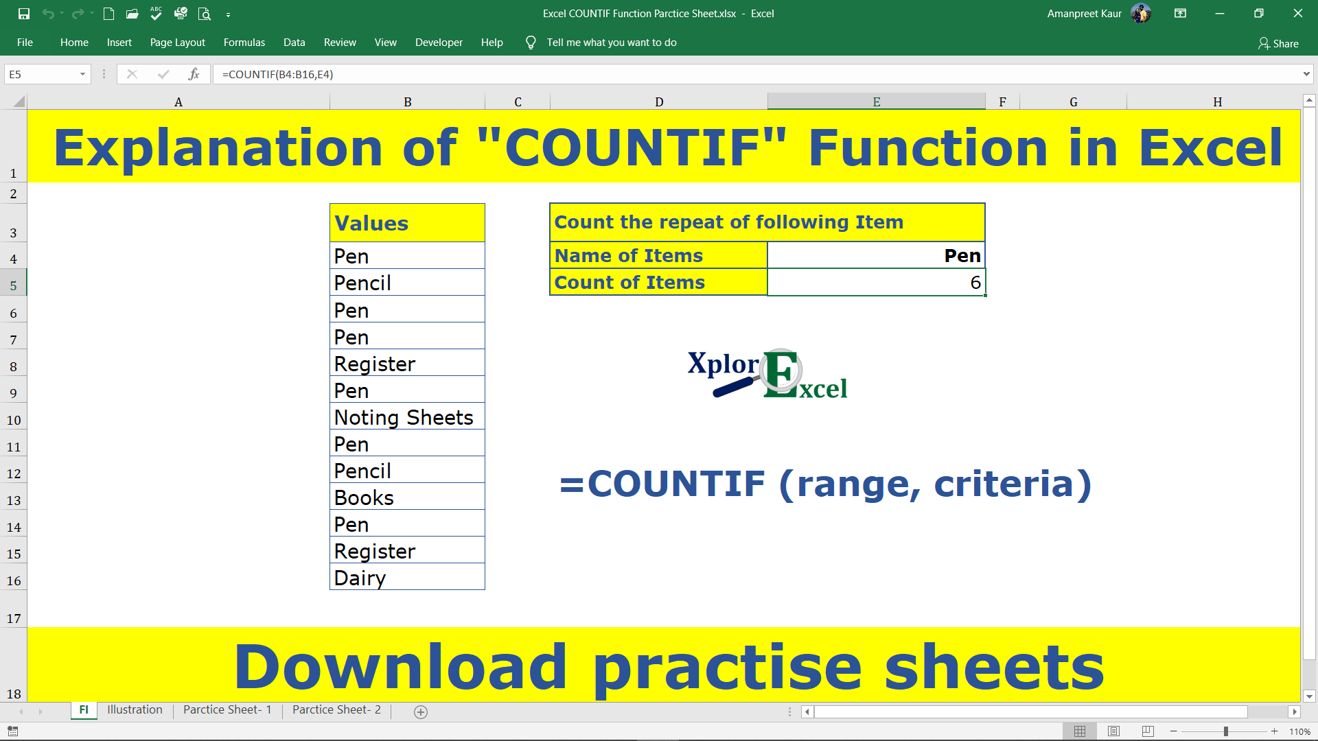
- COUNTIF Excel Function – Download Practice Sheet





[…] Excel SUMIF Function – Download practice Sheet […]
[…] Excel SUMIF Function – Download practice Sheet […]
[…] Excel SUMIF Function – Download practice Sheet […]
[…] Excel SUMIF Function – Download practice Sheet […]
[…] Excel SUMIF Function – Download practice Sheet […]
[…] Excel SUMIF Function – Download practice Sheet […]
how can i download sumifs function practice sheet. pls guide me or send me the link pls
https://xplorexcel.com/excel-sumif-function/
Please check it now:
https://xplorexcel.com/excel-sumif-function/
Please check it now
[…] Excel SUMIF Function – Download practice Sheet […]
ok
thanks
good
Thanks alot
How to download the practice sheets?
Download the Practice Workbook Of SUMIF Function
Please Download Practice workbooks from the below links to know how much you have understood the SUMIF Function in Excel:
SUMIF – Practice Sheet- 1 Download (please click on download word)
SUMIF Practice Sheet- 2 Download (please click on download word)
Im getting wrong value in the 5th
row
How please emailed me the error sheet on xplorexcel21@gmail.com
I’m also facing same issue in both the practice sheets. Value for the fifth item is showing wrong after pasting the formula.
it is working properly please share screenshot with me on my WhatsApp 8725972100
Advertisement-X