How to use VLOOKUP in Excel – Download 5 Practice Sheets for Vlookup.

After reading this article you will be able to use the Vlookup formula to retrieve the data from another table. and you will also get the Free Downloadable Excel practice sheets for the Vlookup formula.

What is VLOOKUP: –

In VLOOKUP, V stands for vertical, and with the help of this formula, we can retrieve the matched value from the selected cells(table array) from left to right means in vertical order. It supports approximate and exact-matched values. It can only look up and retrieve the values in the vertical order. The lookup value must be in the first column in the selected cells(table array).

Need for VLOOKUP formula: –

• With the help of VLOOKUP, we can retrieve the numbers of exact or approximate matched values in seconds.
• It helps save time and do work more efficiently.
• it will show the matched value in the column/row where you want. So, we do not need to find the values individually from the selected date and then copy, and paste it.

The Feature of VLOOKUP formula: –

1. It works only from left to right. It can only look up the value from the Selected cell(Table_array) from left to right side.
2. This formula provides two types of matched values i.e. approximate and exact.
3. VLOOKUP always finds the first matched value from the selected cell(Table_array) and retrieves it.
4. We can use 1 and 0 instead of True and False respectively.
5. It retrieves data based on column numbers.

How to use HLOOKUP in Excel:-

Explanation of VLOOKUP Formula:-

Now, We will explain the Arguments of the formula.

=VLOOKUP(lookup_value, table_array, col_index_num, [range_lookup])

lookup_value: –  The lookup value is that value, which will find the exact matched value from the selected cells(table array) with this formula. This value is always written in the first column of the selected cells(table array) because VLOOKUP only finds the value in the vertical order from the selected cells.

table_array: – This is the array of selected cells from which the VLOOKUP will find and retrieve the matched value.

col_index_num: – It means Column Index Number. The number of that column from which we want to retrieve the matched value. The number of columns is counted from the first column of the selected cells(table array).

range_lookup: – It means what type of match you want to show. There are two types of matches shown as follows: –

1. Ture: – Approximate Match
2. False: – Exact Match

If you want to retrieve the Exact match value to show write the false and if you approximate match then write true.

Example of Vlookup Formula: –

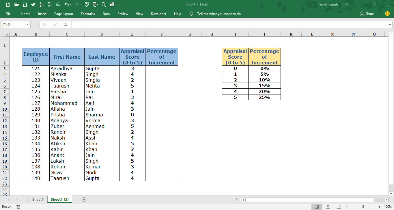
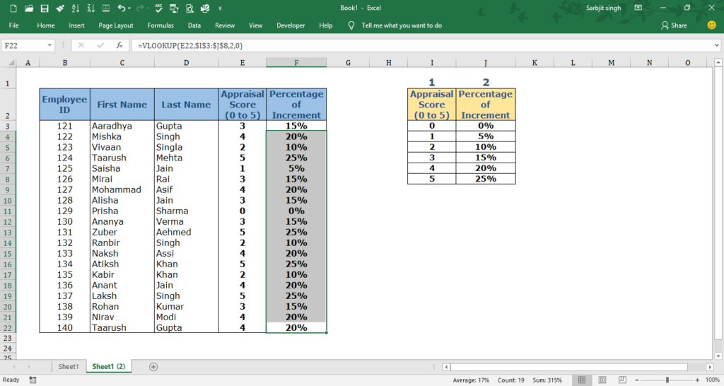
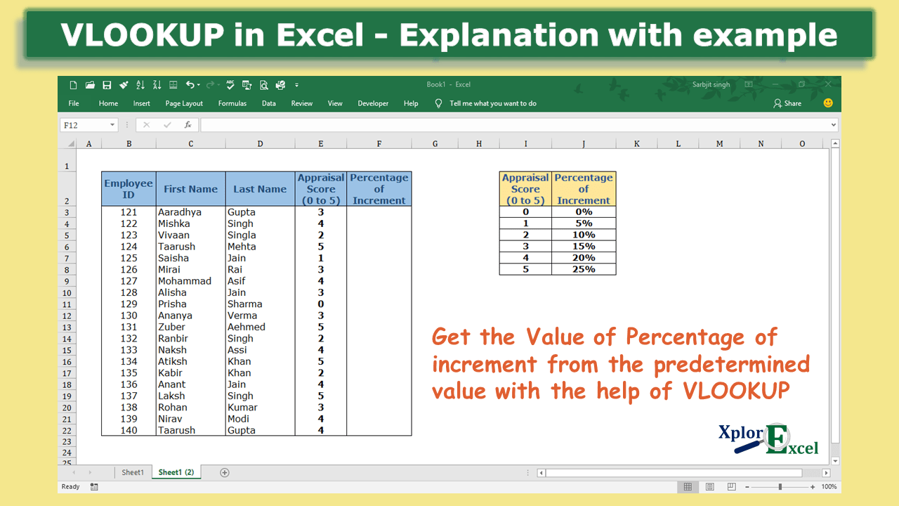
In the following table, we want to retrieve the predetermined percentage of increment from the table according to the appraisal score of each employee.

Solution:-

We will use the VLOOKUP formula to retrieve the predetermined percentage of increments according to the appraisal score of each employee.

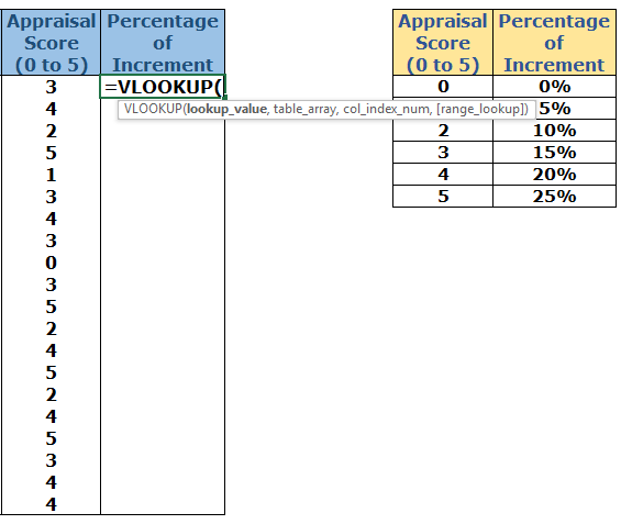
1st Step: –

To use the formula of Vlookup, We have to write the value of cell f3 “=VLOOKUP( “. F3 cell is shown the percentage of increment which we are trying to retrieve from the given table.

2nd Step: – 

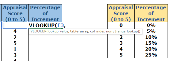
Select the common value in both tables, i.e., the column that consists of Appraisal Score contains the same values in both tables and then after selecting that cell, please add a comma at the end.

=VLOOKUP(E3,

3rd Step: – 

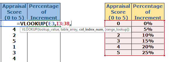
Select the Table array from which you want to retrieve the value then add a comma at the end.

4th Step: –

If you want to Fix the selection of the table array then add the dollar sign ($) at the start and end of the selection shown below: –

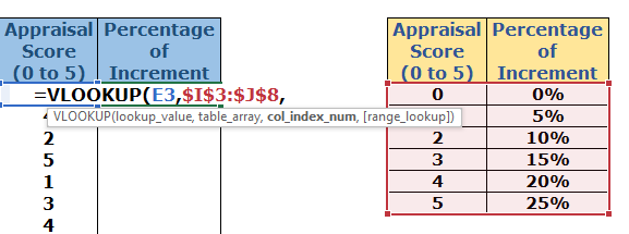
This step is needed when we do not want to update the table array selection when we copy the whole formula in the remaining cell.

5th Step: – 

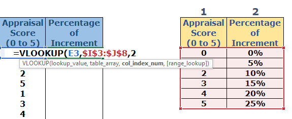
Now select the number of the column of the table array chosen of which the value you want to retrieve.

6th Step: –

Now choose the mode of matching if you want to match the exact value then enter false or 0 otherwise if you want to match the approximate value then enter true or 1. Then after closing the brackets.

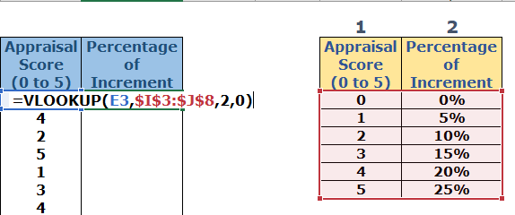
Now, the formula is complete and you will get the result. 

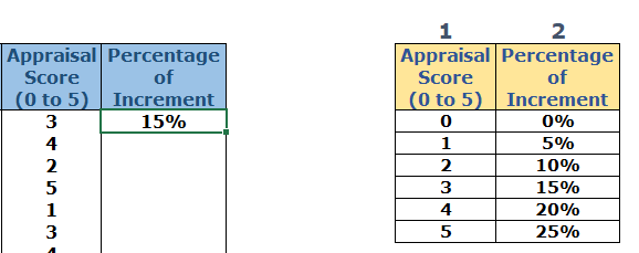
Step No. 7: –

So Now to get the percentage of increment of each employee just copy this result from the f3 cell (means formula) and then paste it in the remaining cell in which you want to use the same.

Download 5 Practice Sheets for Vlookup Formula:

To understand the use of Excel formulas you have to practice it so many times. So that is why we are providing you the Practice sheet for the Vlookup formula free of cost. All major course authors charge so many charges to provide you with the practice sheets. So don’t worry now we are here to provide you for free of cost.

Download the 1st Practice workbook for Vlookup Formula:

Download the 2nd Practice workbook for Vlookup Formula:

Download the 3rd Practice workbook for Vlookup Formula:

Download the 4th Practice workbook for Vlookup Formula:

Download the 5th Practice workbook for Vlookup Formula:

Thanks 

Please Share and comment your feedback in the comment box.

to buy Microsoft Excel Click Here.

Also, Check out the following function of Excel: – 

• HLOOKUP in Excel – Explanation with example
• IF Function in Excel – Explanation with example
• Excel Index Function – Download Practice Sheet
• Excel Match Function- Download Practice Sheet
• Excel SUMIF Function – Download Practice Sheet
• COUNTIF Excel Function – Download Practice Sheet