The “SUMIFS” function is used to know the total of the particular item from the given data with multiple criteria.
What is the “SUMIFS” Function?
The Excel “SUMIFS” function is used when we need to sum up the value on multiple criteria. For example, If we have given the total sale of all products within India, From this data we can use two criteria to get the total sale of pens in the state of Punjab. It is possible only with the “SUMIFS” formula. It can be sum up the value of the cells based on a condition of any Text, number, and logical text. It is also working on matching concepts like VLOOKUP and HLOOKUP but with a condition.
The feature of the “SUMIFS” function: –
- With the help of the “SUMIFS” function, we can retrieve the total of a particular item from the given data if the conditions are matched with the data of the selected cell.
- It helps in applying Two or more conditions to the given data to get the total value of a single item.
The logical operator: –
For the “SUMIFS” function we can also use follow logical test on the selected data other than the Text and Number.
| Logical Test | Meaning |
| = | Equal to |
| <> | Not Equal to |
| > | Greater than |
| >= | Greater than and Equal to |
| < | Less than |
| <= | Less than and equal to |
Explanation of Function:-
Now, We will explain the Arguments of the Function.
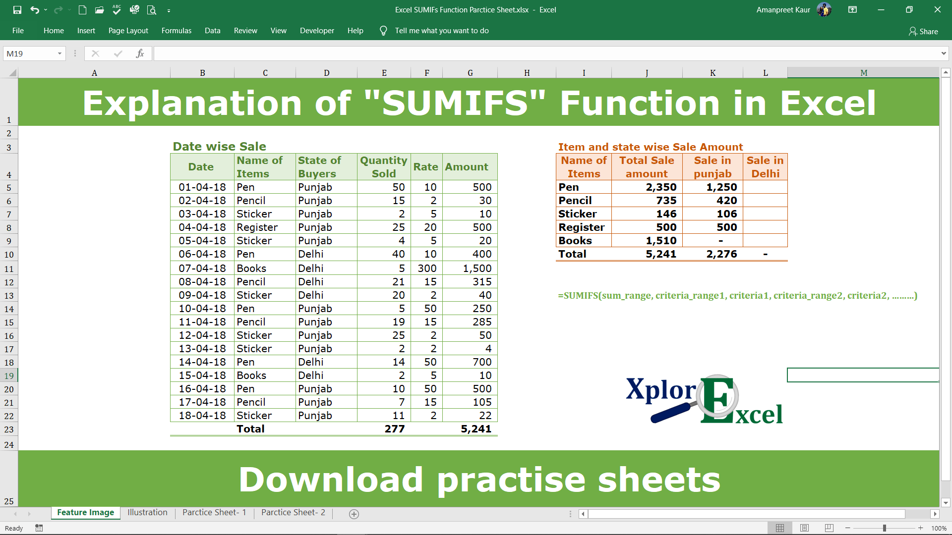
=SUMIFS(sum_range, criteria_range1, criteria1, criteria_range2, criteria2, ………)
sum_range: – Sum range is that range of selected cells, consisting of the values we want to total or sum up.
criteria_range1: – criteria_range1 is that column or row of selected cells on which we want to apply the condition or criteria.
criteria1: – This is a condition that we have to apply to the selected criteria_range1.
criteria_range2[option]: – criteria_range2 optional is that column or row of selected cells on which we want to apply the condition or criteria.
criteria2[option]: – criteria2 is an optional condition that we have to apply to the selected criteria_range2.
Example of Function of SUMIFS: –
I will show you, how to apply the whole function. (using optional also).
From the following table get the item-wise value of the total sale amount.
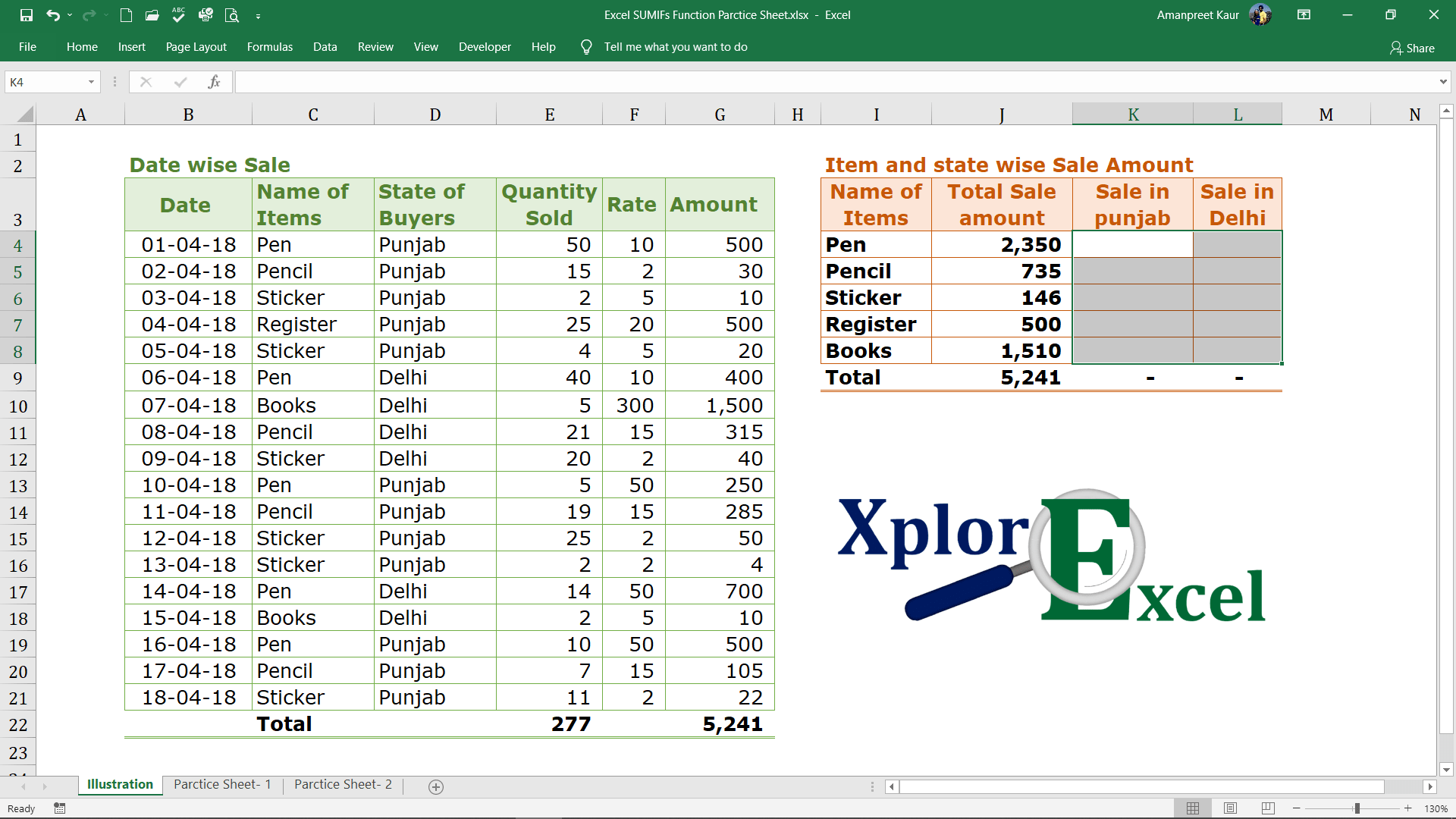
Solution:-
We will Apply the ‘SUMIFS’ function and get the result. This is shown in the following steps: –
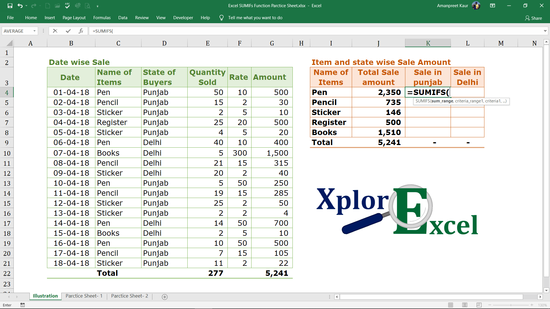
Step No. 1:-
We will write the “=SUMIFS( ” in the column of the result.
Step No. 2
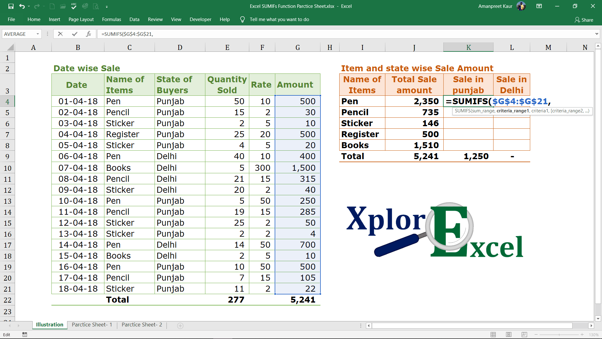
Now select the range on which you want to apply the Condition or criteria.
In an example, we have to sum up the sale amount as per the name of the item. So, we have to apply a condition to the name of the items.

Step No. 3
Now press “F4” to fix the range. it will convert from the G4:G21 to $G$4:$G$21. Now, when you copy this formula in another cell, the range remains the same from the excel will determine the condition or criteria.
Step No. 4
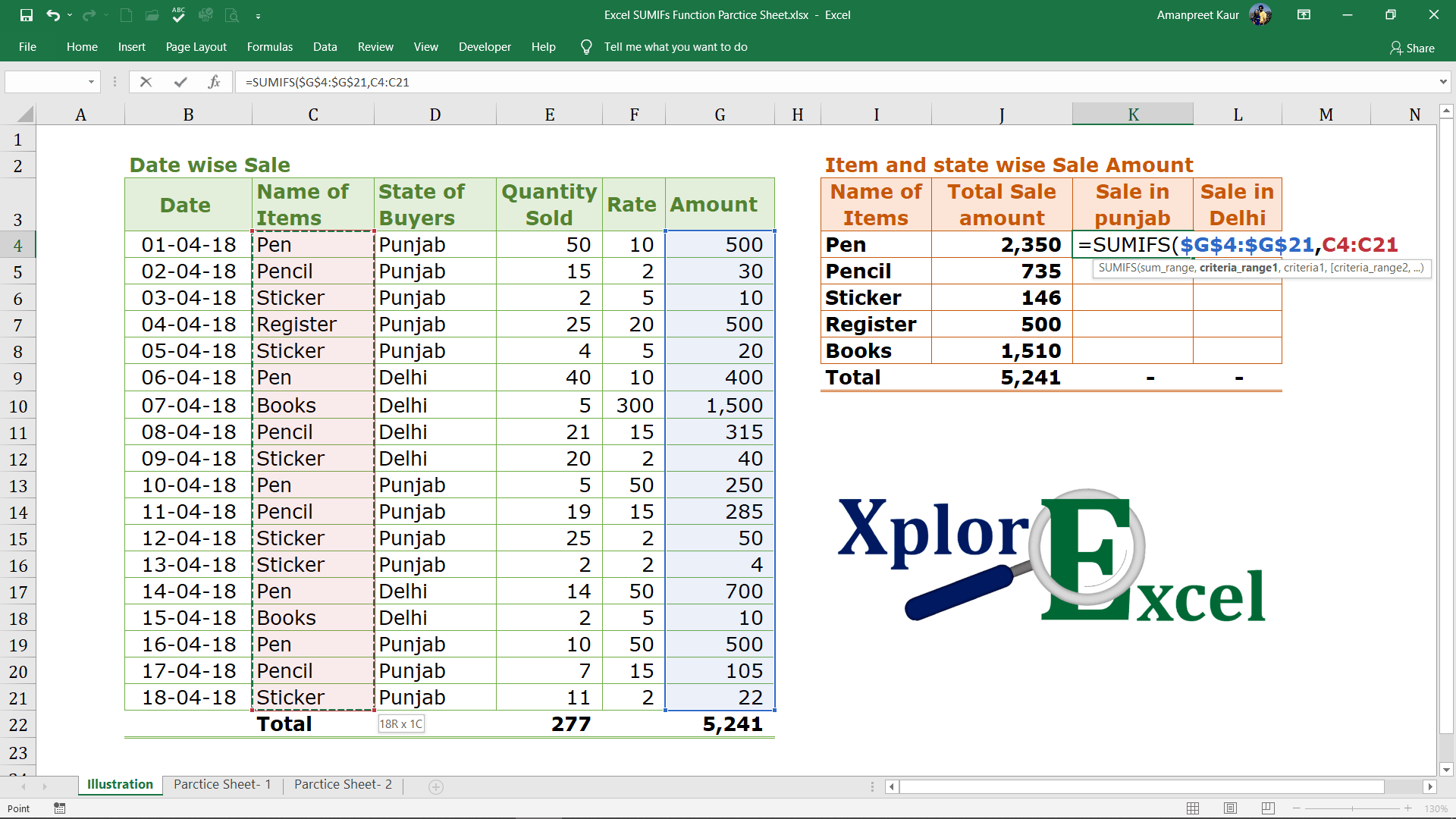
Now select the 1st criteria_range on which we want to apply the 1st criteria or condition.
For example, We want to know the total sale of a specific item. The names of items are given, So we can select the criteria by selecting the range of the names of items.
Step No. 5
Now press “F4” to fix the range. it will convert from the F4:F21 to $F$4:$F$21. Now, when you copy this formula in another cell, the range remains the same from the excel will determine the condition or criteria.
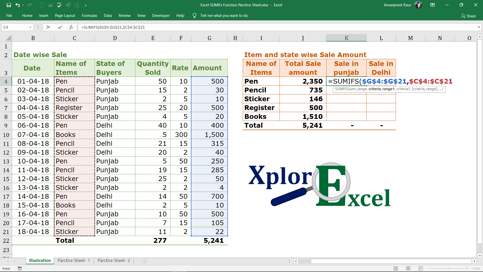
Step No. 6
Now, select the 1st condition or criteria which you want to apply on the 1st criteria_range:
For example, We want to know the total sale of the selected item named Pen. So select the cell that consists of the name of items i.e. column “I”
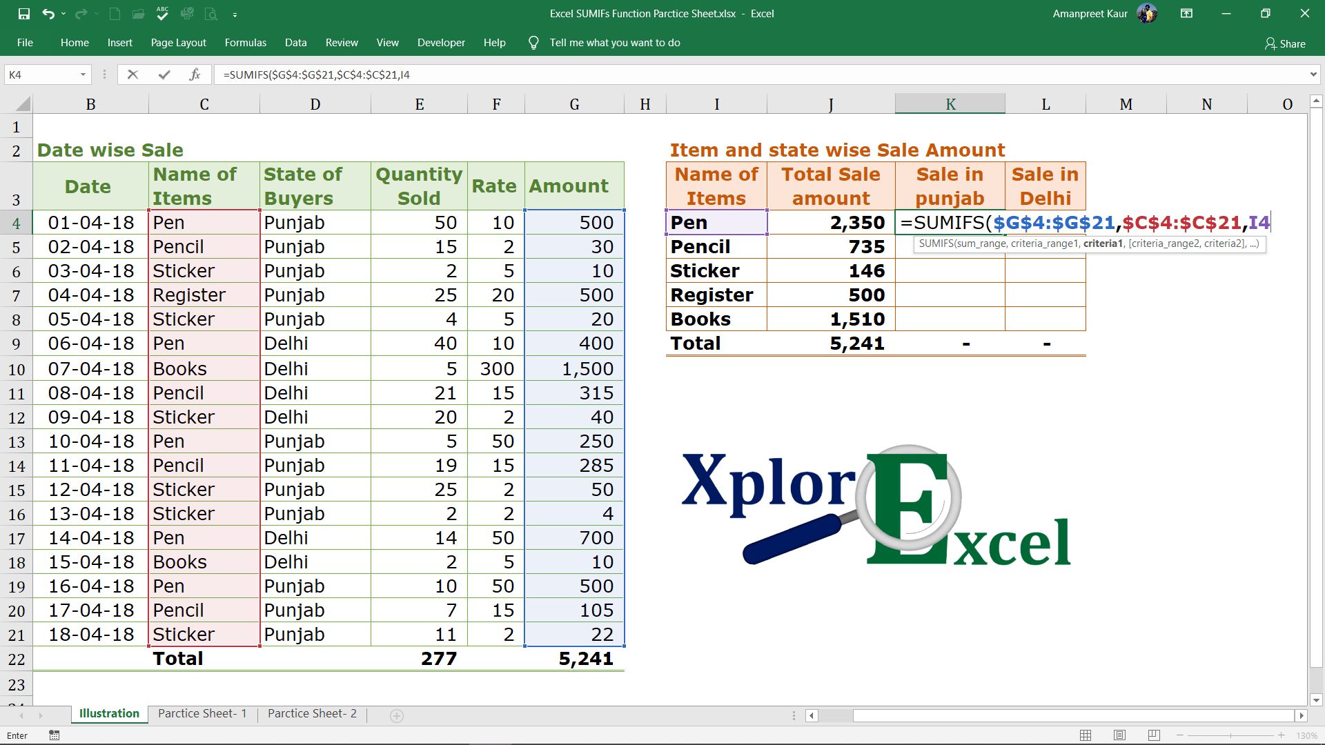
Step No. 7: –
Now select the 2nd criteria_range on which we want to apply the 2nd criteria or condition.
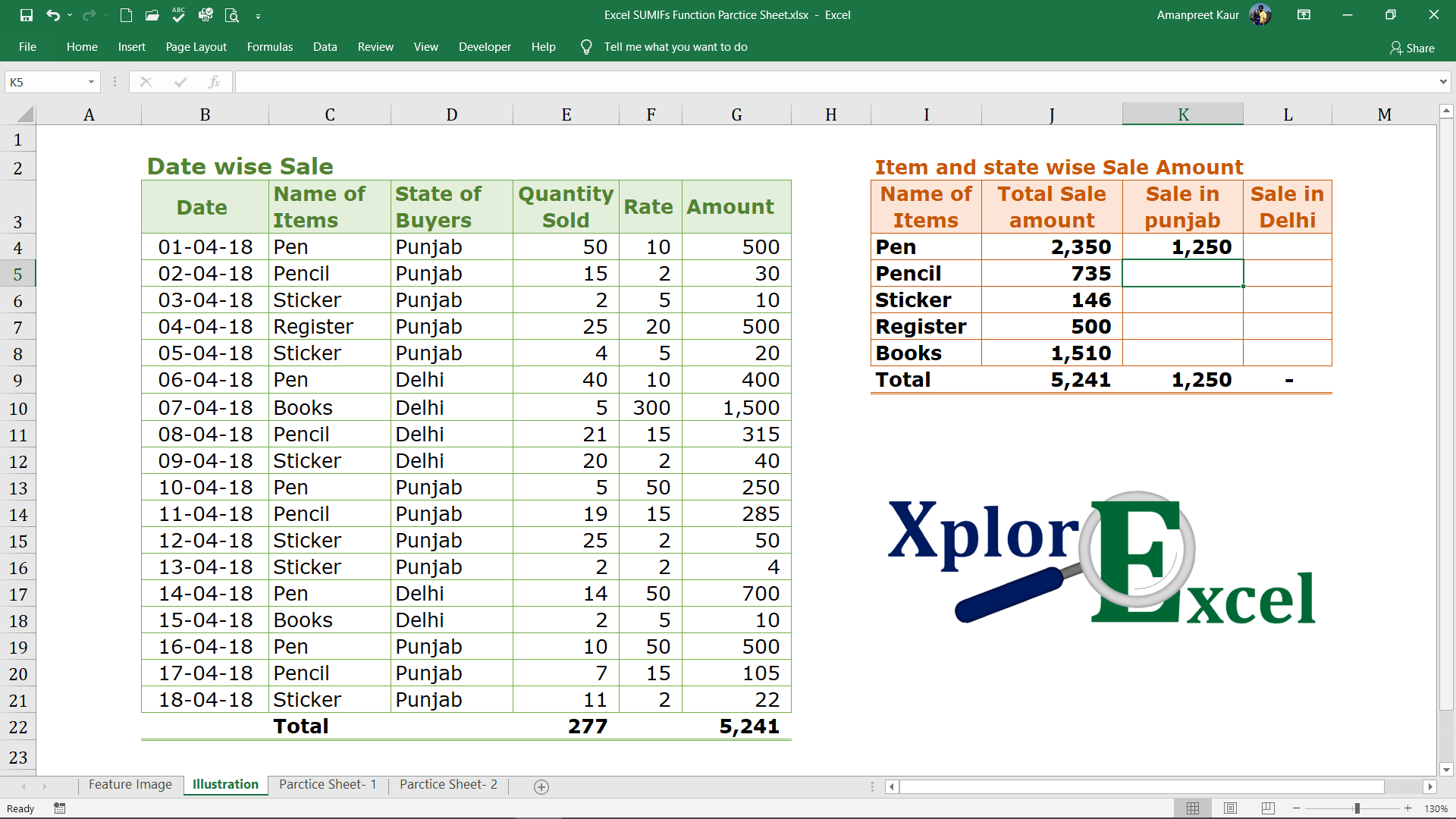
For example, we want to know the total sale of a specific item in a specific area. The name of the area (State) is given in column “D.” So, we can select the second criteria_range by selecting the range of the name of the area(state).
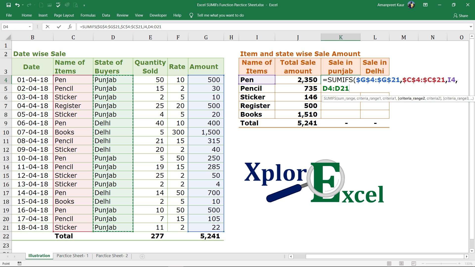
Now press “F4” to fix the range. it will convert from the D4:D21 to $D$4:$D$21. Now, when you copy this formula in another cell, the range remains the same from the excel will determine the condition or criteria.
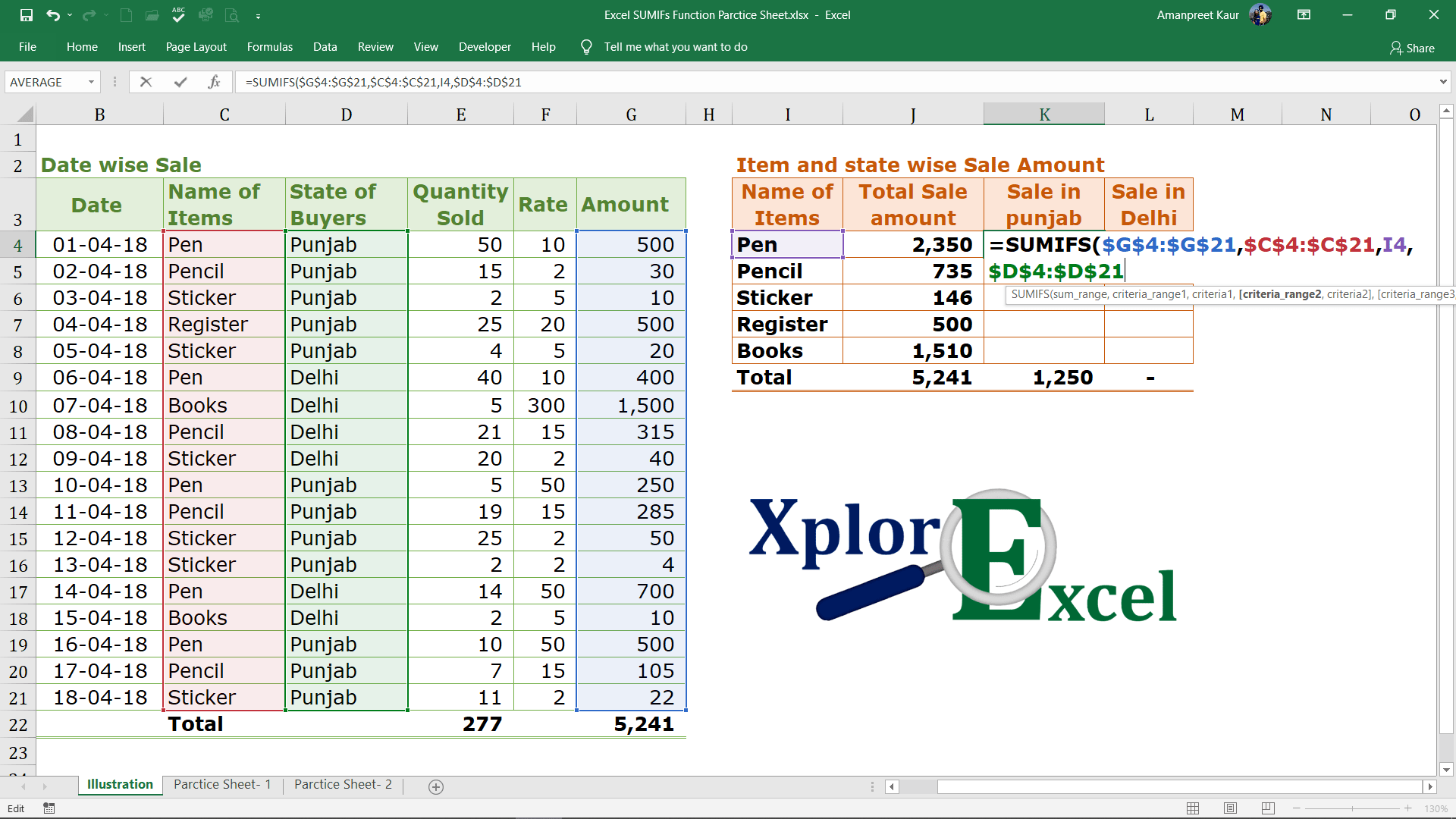
Step No. 9
Now, select the 2nd condition or criteria which you want to apply on the 2nd criteria_range:
For example, We want to know the total sales of the selected item in the specific area, i.e. Punjab. So choose the cell that consists of the name of Area otherwise write it in the invited commas like “Punjab”

Step No. 10
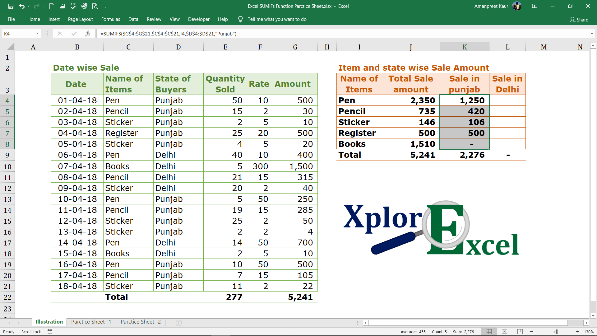
Now, you will get the “SUM” total sale amount of the item named “Pen” in the Punjab:
Step No. 11: –
Now, Copy and paste the function in all remaining cells which are given with the items name to get the result for all items.
Thanks
Please Share and comment on your feedback in the comment box.
to buy Microsoft Excel Click Here.
Also, Check out the following function of excel: –
- How to use VLOOKUP in Excel – free explanation
- How to use HLOOKUP in Excel – free explanation
- IF Function in Excel – Free Explanation with example
- Excel SUMIF Function – Download Practice Sheet
- Excel Match Function- Download Practice Sheet
- Excel Index Function – Download Practice Sheet
- COUNTIF Excel Function – Download Practice Sheet


wow! just wow! Amazing I mean everything is just perfect. detailed explanation of every concept, neat and clean and the illustration helps a lot for better understanding. Thank you! for this detailed content. It really helps me to explore excel more in detail.
Thanks alot.
Please stay tuned we will publish a lot of content on it.
This is very detailed and helps an excel learner to understand the concepts in detail. Thanks for this content.
Most Welcome and thanks for feedback.
can you guide how to download file for practice, i can’t
just click on download button.
Advertisement-X