How to use HLOOKUP in Excel – Download free 5 Practice Sheets For Hlookup.

After reading this article you will be able to use the Hlookup formula to retrieve the data from another table. and you will also get the Free Downloadable Excel practice sheets for the Hlookup formula.

What is HLOOKUP in Excel:

In the HLOOKUP Function “H” stands for horizontal and with the help of this formula, we can retrieve the matched value from the selected cells(table array) from up to down means in horizontal order. It supports approximate and exact-matched values. It can only look up and retrieve the values in the horizontal order. The lookup value must be in the first row in the selected cells(table array).

Need for HLOOKUP formula: –

• With the help of HLOOKUP, we can retrieve the numbers of exact or approximate matched values in seconds.
• It helps in saving time and doing work more efficiently.
• it will show the matched value in the column/row where you want. So, we don’t need to find the values individually from the selected date and then copy, and paste it.

The Feature of HLOOKUP formula: –

1. It works only up to down. It can only look up the value from the Selected cell(Table_array) from up to the downside. it means from the rows.
2. This formula provides two types of matched values i.e. approximate and exact.
3. HLOOKUP always finds the first matched value from the selected cell(Table_array) and retrieves it.
4. We can use 1 and 0 instead of True and False respectively.
5. It retrieves data based on the Row number.

Now, We will explain the Arguments of the formula.

How to use HLOOKUP in Excel:-

Check out how to use HLOOKUP in Excel to do your daily routine work smoothly and efficiently.

Explanation of HLOOKUP Formula:-

Now, We will explain the Arguments of the formula.

=HLOOKUP(lookup_value, table_array, row_index_num, [range_lookup])

lookup_value: –  The lookup value is that value, which will find the exact matched value from the selected cells with this formula. This value is always written in the first row of the selected cells(table array) because HLOOKUP only finds the value in the horizontal order from the selected cells(table array).

table_array: – This is the array of selected cells from which the HLOOKUP will find and retrieve the matched value.

row_index_num: – It means Row Index Number. The number of that row from which we want to retrieve the matched value. The number of rows is counted from the first row of the selected cells(table array).

range_lookup: – It means what type of match you want to show. There are two types of matches shown as follows: –

1. Ture: – Approximate Match
2. False: – Exact Match

If you want to retrieve the Exact match value to show, then write the false and if you approximate the matched value, then write true.

Example of Formula use HLOOKUP in Excel: –

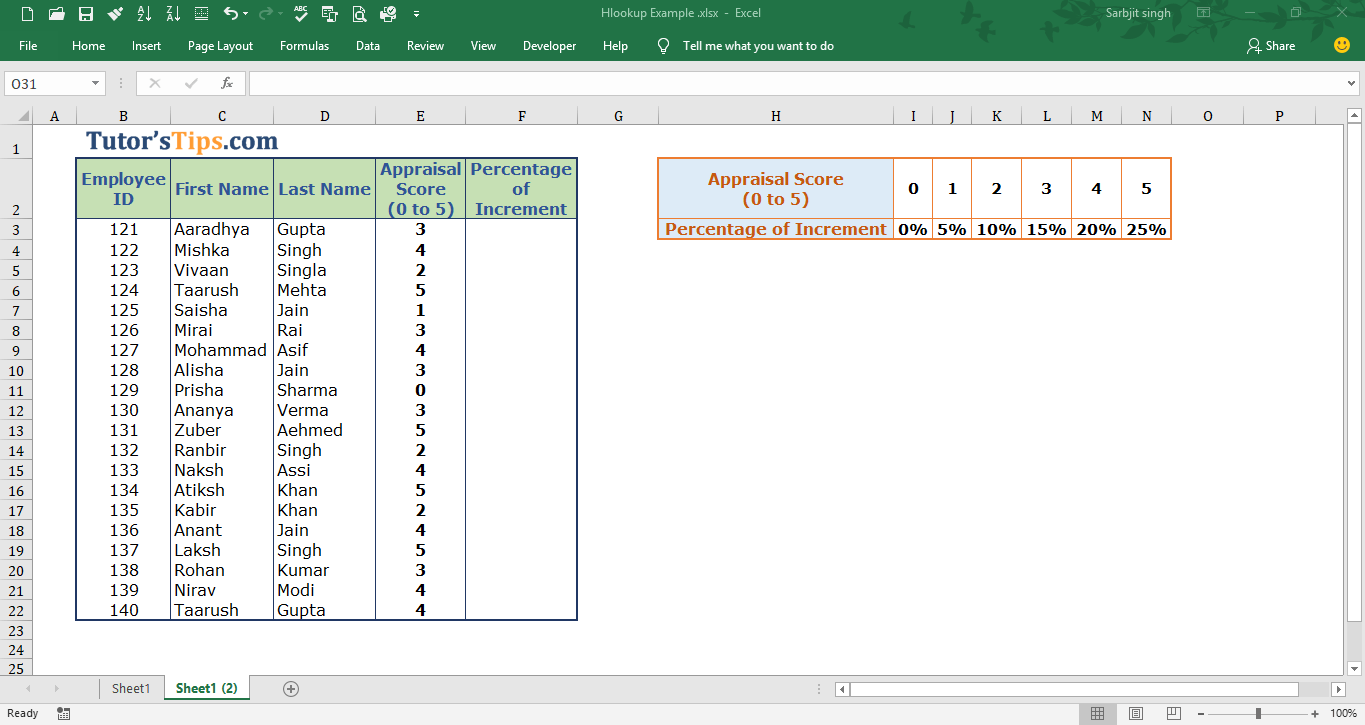
In the following table, we want to retrieve the predetermined percentage of increment from the table according to the appraisal score.

Solution:-

We will use the VLOOKUP formula to retrieve the predetermine the percentage of increment according to the appraisal score.

1st Step: –

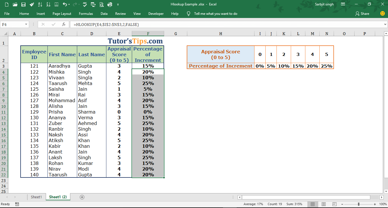
We will write the “=HLOOKUP( ” in the column of the percentage of increment.

2nd Step: – 

Select the value that we common in both tables i.e. Appraisal Score and add a comma at the end.

3rd Step: – 

Select the Table array from which we want to retrieve the value and add a comma at the end.

4th Step: – 

Fix the selection of the table array by adding the dollar sign ($) at both the starting and end of the selection shown below: –

This step is needed when we do not want to update the selection of the table array when we copy the whole formula in the remaining cell. 

5th Step: – 

Now select the number of the column of the selected table array of which the value you want to retrieve.

6th Step: –

Now choose the mode of matching if you want to match the exact value then enter false or 0 or if you want to match the approximate value then enter true or 1.

Now, press the enter key, the formula is complete and you will get the result. 

Step No. 7: – 

So copy this result(means formula) and then paste it in the remaining cell in which you want to use the same.

Download free 5 Practice Sheets For Hlookup Formula:

To understand the use of Excel formulas you have to practice it so many times. So that is why we are providing you the Practice sheet for the Vlookup formula free of cost. All major course authors charge so many charges to provide you with the practice sheets. So don’t worry now we are here to provide you for free of cost.

• Download the 1st Practice workbook for the Hlookup Formula:
• Download the 2nd Practice workbook for the Hlookup Formula:
• Download the 3rd Practice workbook for the Hlookup Formula:
• Download the 4th Practice workbook for the Hlookup Formula:
• Download the 5th Practice workbook for the Hlookup Formula:

Thanks 

Please Share and comment your feedback in the comment box.

to buy Microsoft Excel Click Here.

Also, Check out the following function of Excel: –

• How to use VLOOKUP in Excel – free explanation
• IF Function in Excel – Explanation with example
• Excel Index Function – Download Practice Sheet
• Excel Match Function- Download Practice Sheet
• Excel SUMIF Function – Download Practice Sheet
• COUNTIF Excel Function – Download Practice Sheet